The aim of the ‘bscui’ R package is to render any SVG image as an interactive figure and convert identified elements into an actionable interface. This figure can be seamlessly integrated into ‘rmarkdown’ and ‘Quarto’ documents, as well as ‘shiny’ applications, allowing manipulation of elements and reporting actions performed on them.
Here are the main features of ‘bscui’ figures:
- Interactive view: pan, zoom in/out
- Update the style (e.g., color, stroke, opacity…) of SVG elements
- Update the attribute (e.g., path) of SVG elements
- Export the figure in SVG or PNG format
- Display contextual information when hovering over SVG elements
- Select one or multiple SVG elements (mainly used with ‘shiny’)
- Click on elements (mainly used with ‘shiny’)
- Add or remove SVG elements (in ‘shiny’)
The main motivation behind the development of this package was to be able to leverage SVG images kindly shared in public knowledge resources (e.g., EBI anatomograms, SwissBioPics, or wikipathways ) to display and browse information in the relevant contexts.
The package comes with several pre-processed examples used to demonstrate the main available features described in this document.
Installation and requirements
The ‘bscui’ R package is available on CRAN.
install.packages('bscui')Development version from github
The development version is available in github.
## Dependencies
install.packages("htmlwidgets")
## Install from github
devtools::install_github("patzaw/bscui")
Vignette requirements
The following packages are not dependencies of ‘bscui’ strictly speaking but are required to run code examples discussed in this document.
library(bscui)
library(xml2)
library(dplyr)
library(readr)
library(stringr)
library(glue)
library(scales)
library(reactable)
library(reactable.extras)Built on 2025-04-10
## R version 4.4.1 (2024-06-14)
## Platform: x86_64-pc-linux-gnu
## Running under: Ubuntu 22.04.5 LTS
##
## Matrix products: default
## BLAS:   /usr/lib/x86_64-linux-gnu/openblas-pthread/libblas.so.3
## LAPACK: /usr/lib/x86_64-linux-gnu/openblas-pthread/libopenblasp-r0.3.20.so;  LAPACK version 3.10.0
##
## locale:
##  [1] LC_CTYPE=en_US.UTF-8       LC_NUMERIC=C
##  [3] LC_TIME=en_US.UTF-8        LC_COLLATE=en_US.UTF-8
##  [5] LC_MONETARY=en_US.UTF-8    LC_MESSAGES=en_US.UTF-8
##  [7] LC_PAPER=en_US.UTF-8       LC_NAME=C
##  [9] LC_ADDRESS=C               LC_TELEPHONE=C
## [11] LC_MEASUREMENT=en_US.UTF-8 LC_IDENTIFICATION=C
##
## time zone: Europe/Rome
## tzcode source: system (glibc)
##
## attached base packages:
## [1] stats     graphics  grDevices utils     datasets  methods   base
##
## other attached packages:
## [1] scales_1.3.0  glue_1.8.0    stringr_1.5.1 readr_2.1.5   dplyr_1.1.4
## [6] xml2_1.3.8    bscui_0.1.6   knitr_1.50
##
## loaded via a namespace (and not attached):
##  [1] jsonlite_2.0.0    compiler_4.4.1    tidyselect_1.2.1  jquerylib_0.1.4
##  [5] systemfonts_1.2.2 textshaping_1.0.0 yaml_2.3.10       fastmap_1.2.0
##  [9] R6_2.6.1          generics_0.1.3    htmlwidgets_1.6.4 tibble_3.2.1
## [13] desc_1.4.3        munsell_0.5.1     bslib_0.9.0       pillar_1.10.2
## [17] tzdb_0.5.0        rlang_1.1.5       cachem_1.1.0      stringi_1.8.7
## [21] xfun_0.52         fs_1.6.5          sass_0.4.9        cli_3.6.4
## [25] pkgdown_2.1.1     magrittr_2.0.3    digest_0.6.37     rstudioapi_0.17.1
## [29] hms_1.1.3         lifecycle_1.0.4   vctrs_0.6.5       evaluate_1.0.3
## [33] ragg_1.3.3        colorspace_2.1-1  rmarkdown_2.29    tools_4.4.1
## [37] pkgconfig_2.0.3 htmltools_0.5.8.1- xml2 is used to read SVG files
- readr and dplyr are used to read and manipulate tables with figure contextual information
- stringr and glue are used to facilitate the creation of html tags
- scales is used to generate color scales
- reactable and reactable.extras are used to manipulate information in a table displayed in the Shiny example
Building figures
The main function of the package is bscui(). It takes as
main argument a character string with SVG code. The use of xml2 to read SVG
files is not mandatory but it can be useful to validate the SVG and
manipulate it before displaying it.
Simple example: Animal cells
This example relies on a figure of animal cells taken from SwissBioPics.
svg <- xml2::read_xml(system.file(
   "examples", "Animal_cells.svg.gz",
   package="bscui"
))
The simplest way to display the figure is shown below.
figure <- bscui(svg)
figure
The figure can be grabbed with mouse and enlarged or shrunk using the mouse wheel. Clicking on the button at the top-left corner of the figure displays a menu with various functions, including resetting the view and exporting the figure in SVG or PNG format. Several configuration choices are made by default but can be changed, such as the zoom range or the width of the menu.
Defining UI elements
User Interface (UI) elements are provided as a data frame with the following columns:
- id: the element identifier
- ui_type: either “selectable” (several elements can be selected), “button” (action will be triggered by clicking), “none” (no action on click)
- title: a description of the element to display when the mouse hovers over the element
Information about the different part of a cell were taken from UniProt.
info <- readr::read_tsv(system.file(
   "examples", "uniprot_cellular_locations.txt.gz",
   package="bscui"
), col_types=strrep("c", 6)) |>
   mutate(id = str_remove(`Subcellular location ID`, "-"))
The title feature can take simple text or a valid html element as shown below.
ui_elements <- info |>
   mutate(
      ui_type = "selectable",
      title = glue(
         '<div style="width:300px; height:100px; overflow:auto; padding:5px;',
         'font-size:75%;',
         'border:black 1px solid; background:#FFFFF0AA;">',
         "<strong>{Name}</strong>: {Description}",
         "</div>",
         .sep=" "
      )
   ) |>
   select(id, ui_type, title)
ui_elements
## # A tibble: 563 × 3
## id ui_type title
## <chr> <chr> <glue>
## 1 SL0002 selectable <div style="width:300px; height:100px; overflow:auto; padd…
## 2 SL0003 selectable <div style="width:300px; height:100px; overflow:auto; padd…
## 3 SL0004 selectable <div style="width:300px; height:100px; overflow:auto; padd…
## 4 SL0005 selectable <div style="width:300px; height:100px; overflow:auto; padd…
## 5 SL0006 selectable <div style="width:300px; height:100px; overflow:auto; padd…
## 6 SL0007 selectable <div style="width:300px; height:100px; overflow:auto; padd…
## 7 SL0008 selectable <div style="width:300px; height:100px; overflow:auto; padd…
## 8 SL0009 selectable <div style="width:300px; height:100px; overflow:auto; padd…
## 9 SL0010 selectable <div style="width:300px; height:100px; overflow:auto; padd…
## 10 SL0011 selectable <div style="width:300px; height:100px; overflow:auto; padd…
## # ℹ 553 more rows
figure <- figure |>
   set_bscui_ui_elements(ui_elements)
figure
Setting element styles
The style of the elements can be changed with the
set_bscui_styles() function. The styles are are provided in
a data frame with an id column, providing the element identifier, and
one column per style. Column names should correspond to a style name in
camel case (e.g., “strokeOpacity”). This function can be called several
times to change different elements or different options.
figure <- figure |>
   set_bscui_styles(
      bind_rows(
         info |>
            filter(Name == "Cytosol") |>
            mutate(fill = "#FF7F7F"),
         info |>
            filter(Name == "Nucleoplasm") |>
            mutate(fill = "#7F7FFF")
      ) |>
         select(
            id, fill
         )
   ) |>
   set_bscui_styles(
      info |>
         filter(Name == "Endosome") |>
         mutate(stroke = "yellow", strokeWidth = "2px") |>
         select(id, stroke, strokeWidth)
   )
figure
Setting element attributes
Element attributes can also be changed with the
set_bscui_attributes() function. The example below shows
how to focus on the nucleus and its content starting from the original
figure, by setting the “display” attribute of all other elements to
“none”. Also the size of the nucleolus is slightly increased.
nucleus_part <- c(
   "SL0191", "SL0190", "SL0182", "SL0188", "SL0494", "SL0180",
   "SL0031", "SL0465", "SL0127", "SL0186"
)
figure <- figure |>
   set_bscui_attributes(
      info |>
         filter(
            !id %in% nucleus_part
         ) |>
         mutate(display="none") |>
         select(id, display)
   ) |>
   set_bscui_attributes(tibble(id="sib_copyright", display="none")) |>
   set_bscui_attributes(tibble(id="SL0188", transform="scale(1.8 1.8)")) |>
   set_bscui_attributes(
      tibble(id="SL0188", transform="translate(-237 -202)"),
      append=TRUE
   )
figure |>
   set_bscui_options(
      show_menu=FALSE, zoom_min=1, zoom_max=1, clip=TRUE,
      hover_width=1
   )
In the example above the set_bscui_options() function is
used to hide the menu and to disable view changes (zoom and pan). Other
options can be changed with this function.
Save and export widget
The htmlwidgets::saveWidget() function can be used to
save the figure in an interactive html file.
bscui(svg) |>
   htmlwidgets::saveWidget(file = "figure.html")
And the export_bscui_to_image() is used to export the
figure as an image.
bscui(svg) |>
   set_bscui_options(show_menu=FALSE) |>
   export_bscui_to_image(file = "figure.png", zoom=6)
This function relies on the ‘webshot2’ package and requires the Chrome browser or other browsers based on Chromium, such as Chromium itself, Edge, Vivaldi, Brave, Opera or Thorium. The following code chunk shows how to rely on Microsoft Edge.
Sys.setenv(
    "CHROMOTE_CHROME" = "C:/Program Files (x86)/Microsoft/Edge/Application/msedge.exe"
)
Mapping data: Wikipathways
The following example demonstrates how to use ‘bscui’ to map numeric data with colors on the figure. In this example, gene expression data are used to color elements of the Principal pathways of carbon metabolism taken from WikiPathways.
svg <- xml2::read_xml(system.file(
   "examples", "WP112.svg.gz",
   package="bscui"
))
info <- read_tsv(system.file(
   "examples", "WP112.txt.gz",
   package="bscui"
), col_types="c")
Gene expression data were taken from a publication describing the effects of the provided nitrogen sources on baker’s yeast gene expression (Godard et al. 2007). The supplementary Table S1 provides a list of genes displaying significant variations in expression under at least one tested nitrogen condition compared to urea.
deg <- read_tsv(system.file(
   "examples", "DEG-by-nitrogen-source_MCB-Godard-2007.txt.gz",
   package="bscui"
), col_types=paste0(strrep("c", 3), strrep("n", 41)))
Below, we focus on the ALANINE condition and extract the M value comparing the expression of genes when this amino-acid is used as the nitrogen source instead of urea in yeast culture: $M = log_2\left(Expression\,on\,alanine \over Expression\,on\,urea\right)$
condition <- "ALANINE"
toTake <- c("ORF", paste(condition, "M"))
cond_deg <- deg |>
   select(all_of(toTake)) |>
   setNames(c("ensembl", "M")) |>
   filter(!is.na(M))
We define a color scale on M values and define the style of the SVG elements accordingly.
col_scale <- col_numeric(
   "RdYlBu", domain=range(cond_deg$M), reverse=TRUE
)
styles <- cond_deg |>
   mutate(
      fill=col_scale(M)
   ) |>
   inner_join(select(info,id, ensembl), by="ensembl") |>
   select(id, fill)
Finally, we create tooltips on SVG elements showing the type of biological object and the M value when available.
elements <- info |>
   mutate(
      ui_type="selectable",
      bg = case_when(
         category == "GeneProduct" ~ "#FDFDBD",
         category == "Metabolite" ~ "#BDFDFD",
         TRUE ~ "white"
      )
   ) |>
   left_join(cond_deg, by="ensembl") |>
   mutate(
      de = ifelse(
         !is.na(M),
         glue("log2({condition}/UREA) = {round(M,2)}<br/>"),
         ""
      )
   ) |>
   mutate(
      title = glue(
         '<div style="padding:5px;border:solid;background:{bg}">',
         '<strong>{name}</strong><br/>',
         '{de}',
         '<a href={href} target="_blank">{category} information</a>',
         '</div>'
      )
   ) |>
   select(id, ui_type, title)
And we use this information to create the figure.
bscui(svg) |>
   set_bscui_ui_elements(elements) |>
   set_bscui_styles(styles)
‘shiny’ applications
The following example is used to describe the capabilities of ‘bscui’ within ‘shiny’. It relies on the human female anatomical diagram taken from the EBI gene expression group.
shiny::runApp(system.file("examples", "shiny-anatomogram", package = "bscui"))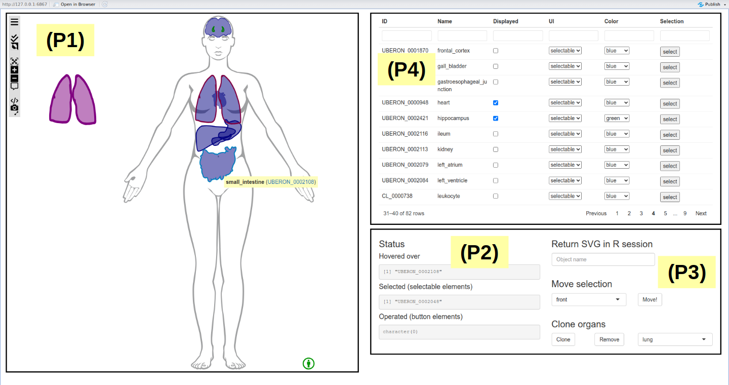
The application is divided in four main parts:
- (P1) On the left: the anatomical diagram
- On the bottom right:
- (P2) text outputs showing the input values that are updated when interacting with the diagram
- (P3) interfaces to modify the anatomical diagram and export it in R session
- (P4) On the top right: a table to choose the organs and configure the interactions
Building and inserting the figure (P1)
Building the figure and inserting it in ‘shiny’ user interface is
straightforward and relies on the bscuiOutput() and
renderBscui() functions:
ui <- fluidPage(
   bscuiOutput("anatomogram")
)
server <- function(input, output, session){
   output$anatomogram <- renderBscui({
      bscui(svg)|>
         set_bscui_ui_elements(ui_elements)
   })
}
UI elements need to be defined with
set_bscui_ui_elements() to make the figure interactive and
to allow ‘shiny’ interactions.
Interactions (P2)
The following information are exposed to ‘shiny’ from the ‘bscui’ widget:
-
input$bscuiID_selectedreports selected elements -
input$bscuiID_operatedreports operated button elements -
input$bscuiID_hoveredreports hovered elements
bscuiID is used to refer to the figure output id,
“anatomogram” in the example above.
Modifying the figure (P3)
Creating a “bscui_Proxy” object allows figure modification without
redrawing it. It’s done by calling the bscuiProxy() within
the sever function:
server <- function(input, output, session){
   output$anatomogram <- renderBscui({
      bscui(svg)|>
         set_bscui_ui_elements(ui_elements)
   })
   anatomogram_proxy <- bscuiProxy("anatomogram")
}
The following functions can then be used to modify the figure:
-
order_bscui_elements()changes the display order of chosen elements -
add_bscui_element()adds an element to the figure -
remove_bscui_elements()removes chosen elements from the figure
Finally, the get_bscui_svg() function makes the updated
figure SVG available via input$bscuiID_svg
(input$anatomogram_svg in the example).
Updating figure elements (P4)
The example above relies on the ‘reactable’ and ‘reactable.extras’
packages to display available elements (organs) and change their
properties. The following functions are applied to a “bscui_Proxy”
(anatomogram_proxy in the example above).
update_bscui_ui_elements()changes the type and the title of elements. It is used in the example above to select the type (“selectable”, “button” or “none”) of each element from the “UI” column.update_bscui_attributes()sets attributes of SVG elements. It is used in the example above to display or hide the different organs from the “Displayed” column.update_bscui_styles()sets styles of SVG elements. It is used in the example above to modify the color of the organs from the “Color” column.update_bscui_selection()updates the list of selected elements. In the example, it is used to select organs from the “Selection” column of the table (organs can therefore be selected either from the table or directly from the diagram).click_bscui_element()triggers a click on a “button” element. It is not used in the example.
Additional notes
The functions of the ‘bscui’ package do their best to handle and modify SVG elements as accurately as possible. However, depending on the structure of the SVG it can be more or less successful. Simple and unnested structures should be preferred when building SVG specifically for this use.
However, the aim of the ‘bscui’ package is also to leverage SVG from existing sources as shown in all the examples described here. The vignette Preparing SVG: examples, tips and tricks describes how the SVG used in ‘bscui’ package examples were prepared. This experience can be used when preparing SVG from new sources.